2D Jacobi Program


      // Assumed variable declarations

      #define THRESHOLD ...

      double inMatrix[N][N] = { ... };

      double outMatrix[N][N];

      double maxDiff;

      

      // Outer-Loop - Keep doing iterations

      do {

      

        // Reset maxDiff

        maxDiff = 0.0;

      

        // Update all values in the matrix ("inner-loop")

        for (int x = 0; x < N; x++) {

          for (int y = 0; y < N; y++) {

      

            // Start with "self" value

            double sum = inMatrix[x][y];

            int divisor = 1;

      

            // Add the neighbors' values to average calculation

            if (x > 0)     { sum += inMatrix[x - 1][y]; divisor++; }

            if (x < N - 1) { sum += inMatrix[x + 1][y]; divisor++; }

            if (y > 0)     { sum += inMatrix[x][y - 1]; divisor++; }

            if (y < N - 1) { sum += inMatrix[x][y + 1]; divisor++; }

      

            // Calculate new value, difference, and update maxDiff

            outMatrix[x][y] = sum / ((double)divisor);

            double diff = abs(inMatrix[x][y] - outMatrix[x][y]);

            if (diff > maxDiff) maxDiff = diff;

          }

        }

      

        // Swap in and out

        double* tmp = inMatrix;

        inMatrix = outMatrix;

        outMatrix = tmp;

      

      } while (maxDiff > THRESHOLD);

Figure 1: C++ Code for 2D Jacobi Calculation

Figure 2: Decomposition of 2D Jacobi (Parallel Data Structure)

Figure 3: Communication Pattern (Single Chare, Single Step)

The Jacobi Calculation

The Jacobi calculation is another useful example. The idea is simple. There is some data set (1D, 2D, 3D, etc. array of values) which is updated in an iterative processes until some condition is met. For this example, we will compute a new value for each element in a 2D matrix. The element's new value will be the average of the element's current value and the current values of its four neighbors. We will do this for every element in the matrix (an iteration). At the end of each iteration, the maximum value change will be determined. That is, for each element in the matrix, the value change is the difference between the old value and the new value. That maximum of all the value changes is calculated across the entire 2D matrix. If the maximum value change for a given iteration is below a given threshold, then the Jacobi calculation ends. Otherwise, the next iteration starts. Figure 1 to the right has the C++ code for a serial version of the 2D Jacobi calculation described above..

Parallelizing 2D Jacobi

There is a lot of potential to parallelize the Jacobi calculation. While each outer-loop iteration requires the output of the previous iteration, each iteration of the outer-loop can be parallelized. Notice the two for-loops (which will collectively be referred to as the inner-loop). Each iteration of the inner-loop writes to a different element of the outMatrix and only reads values from the inMatrix. Because of this, the calculation of each element's new value along with the element's difference (diff value in the code) can be performed in parallel.

Decomposing a Single Outer-Loop Iteration

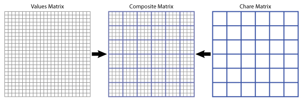
The main decision is how to decompose the iterations of the inner-loop into sets (with the idea being that a single chare object will perform all inner-loop iterations within a single set). For now, we will ignore the code in the inner-loop that updates maxDiff (i.e. "if (diff > maxDiff) maxDiff = diff;"). For this example, we will break down the matrix into blocks (that is several 2D sub-matrices). Each chare object will have a single 2D sub-matrix and perform the corresponding iterations of the inner-loop on those matrix elements. Figure 2 depicts this decomposition visually for the entire matrix.

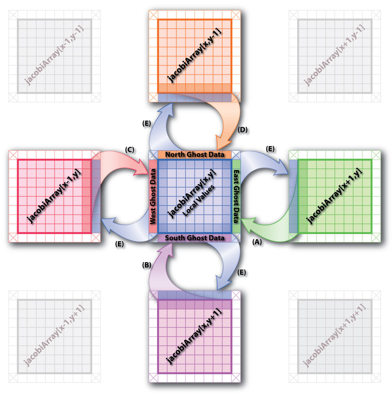
Figure 3 zooms in on a single chare object and the eight surrounding chare objects (assuming the center chare object is not one of the border elements). The jacobiArray refers to a 2D array of Jacobi chare objects (the name used in the example code below). Five events have to occur each step before the chare object can perform its local calculation. They are as follows (Please Note: these events can occur in any order):

A: The chare object to the east (x+1,y) sends its west-most column of data to this chare object (x,y). The data is copied from the message into the east ghost data location.
B: The chare object to the south (x,y+1) sends its north-most row of data to this chare object (x,y). The data is copied from the message into the south ghost data location.
C: The chare object to the west (x-1,y) sends its east-most column of data to this chare object (x,y). The data is copied from the message into the west ghost data location.
D: The chare object to the north (x,y-1) sends its south-most row of data to this chare object (x,y). The data is copied from the message into the north ghost data location.
E: This chare object (x,y) must likewise send out ghost data to each of its four neighbors (assuming it is not a border chare object). This is done in a manner similar to how each of the incoming ghost data messages were sent.

Once each of these events have occurred, the local chare object (x,y) is then ready to do the Jacobi calculation on its local data (similar to the inner-loop calculation in the serial C++ code in Figure 1 except only on the local sub-matrix instead of the entire values matrix). However, the maxDiff value calculated will only be the maxDiff found in the local sub-matrix. The global maxDiff must be calculated from all the local maxDiff values.

Handling maxDiff

The only challenge to parallelizing the inner-loop iterations is the calculation of the maxDiff value. This scalar value is both read and written by each iteration of the inner-loop. However, this is easily overcome if one notices that the operation being performed on the maxDiff variable, maxDiff = max(maxDiff, diff), is both associative and commutative. Because of this, it doesn't matter what order the individual max operations are performed in. As long as they are all performed, the same answer will be reached. Therefor, each chare object in the chare matrix can perform the maxDiff operations local to it. All of the local maxDiff values can then be collected into a single location and then combined using the same max operator.

The type of role maxDiff is playing in this code is a common one in parallel programs in general. This pattern is referred to as a reduction. The Charm++ model and the Charm++ Runtime System have special support for handling reductions of various types (including user-defined reductions). For the sake of this example, we will perform the reduction manually. For more information on using built-in support for reductions within Charm++, please refer to Section 3.14 "Reductions" of The Charm++ Programming Language Manual.

Implement It

Try implementing the 2D Jacobi calculation in Charm++. To get you started, here are some hints that you might find useful:

Makefile: The Makefile for this application should be very similar to the makefiles used in the Array and Broadcast versions of the "Hello World" examples.
Initial Values: Create a chare array and have each chare object initialize its portion of the overall 2D matrix with values of zero. During the calculation, at some code that holds a portion of the values constant. For example, hold inMatrix[0][0] = 1.0 or hold the entire first row's and/or first column's values at 1.0.

Solution

A simple solution for this problem can be found here (Basic2DJacobi.tar.gz).

NOTE: In this solution, there is a "#define DISPLAY_MATRIX" line in the common.h header file which controls whether or not the chare objects will display their portion of the matrix during each step of the calculation. By default, the output is disabled as it can be quite a bit of output depending on the parameters that are used for the application. To see the values in the matrix during each step, set DISPLAY_MATRIX to a non-zero value.

Extensions / Performance Considerations

No Need for Barriers

As was the case with the Parallel Prefix example, the implicit barrier created by contacting the main chare each iteration is not needed. Instead, once the data dependencies created by passing ghost information between the chare objects are satisfied, the chare objects should move forward with their calculations. Implement this code without using barrier during the actual Jacobi calculation. Once again, be careful to consider all the possible race conditions that might occur and verify that your program is indeed producing correct results.