Particles Code with Load Balancing and Performance Analysis

Figure 1

Description

This assignment is an extension of Particles Code. You will use your code from Particles Code and extend it to do load balancing and visualization using LiveViz.

In Particles Code, the particles moved randomly. There was no prominent load imbalance between chare array elements. Now we will create load imbalance between chares by coloring the particles, moving them at different speeds, and changing their initial distribution.

• The particles will have three colors: blue, red, and green. To represent this, you need to add a variable to the Particle object.
• To make particles move at different speeds, add a constant speed factor to the perturb function depending on the color of the objects. Change the range of blue particles to half, red particles will have the full range (so they will move faster), and green particles will move at one-quarter speed.
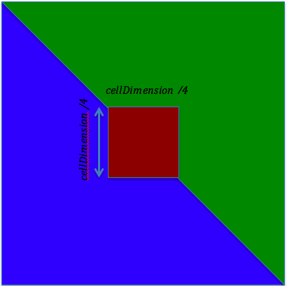
• You are also required to change the initial distribution of the particles depending on the color. In the beginning green particles will be distributed to the right upper triangle, blue particles will be on the left lower triangle of the cell, and red particles will be in the middle square. Chare array elements having red particles will have 2*particlesPerCell number of particles per cell and the rest of the chare array elements will have particlesPerCell number of elements where particlesPerCell is a command line argument as in Particles Code.
• This will result in chares along the diagonal generating both green and blue particles in their bounding box. Thus, they will have 2*particlesPerCell. Additionally, chares along the diagonal inside the red box will generate red particles in addition to the green and blue chares. In total they will have 4 * particlesPerCell (1 (for Green) + 1 (for Blue) + 2 (for Red) * particlesPerCell). The other chares in the red box not on the diagonal will generate both red and green or blue particles. Their total will be 3 * particlesPerCell (2 (Red) + 1 (Green or Blue) * particlesPerCell). See Figure 1.

Part A) Load Balancing and Projections:

In this part, you'll try 3 different load balancing strategies and comment on the behavior you observe. The first two load balancing strategies you will use are GreedyLB and RefineLB. For the third strategy, you will get to choose one of the other load balancing strategies. Observe the effect of load balancing (overhead and benefit) on the total execution time of the application using Projections. Are they beneficial? Why or why not? How much is the overhead? Which strategy is the best for this Particle application? etc.

Part B) Visualization using LiveViz:

In this part you will visualize the 2-D grid with moving particles using LiveViz. Particles should be shown in color. You need to submit two images from the visualization: one in the beginning showing the initial particle distribution and one when the application is more advanced (after the particles are moved and intermixed).

Please read the LiveViz manual for details about LiveViz setup and usage. You can also look at the Wave2D application for an example code that uses LiveViz. It's located in charm/examples/charm++/wave2d.